Magic Formula 6.1 fit over measured tyre data

Built in MATLAB & Simulink Models 19 Team MAC Formula Electric

Model library

Home
9 DOF

Corner balance model

Newest, and the most complex
MATLAB
Simulink
MF 6.1 tyre
26 parameters

Nine degrees of freedom: yaw and sideslip in the plane, heave, roll and pitch of the sprung mass, and the vertical motion of each unsprung corner. Load transfer falls out of the suspension states instead of a steady-state formula, so every tyre sees its own normal load and the Magic Formula returns cornering stiffness at that load, camber and pressure. The two tyres on an axle sum to the axle stiffness that drives the yaw-plane solution, and its lateral acceleration feeds straight back into the load transfer. That loop is the one the simpler models cut.

The nine degrees of freedomSprung-mass heave, roll and pitch at the top; the front and rear unsprung subsystems below. Each returns its own spring and damper force, and each corner carries its own vertical state.
Whole-model architectureFour Magic Formula blocks on the left, one per corner. Their cornering stiffnesses feed the yaw-plane solver on the right, whose lateral acceleration closes the loop back into load transfer.
Axle cornering stiffness, built up per tyreEach tyre's own normal load, camber and pressure go into its own MF 6.3 block. The two outputs sum to the axle stiffness the bicycle solution actually uses.
Understeer gradient through a sine steerBetween -0.028 and -0.038 deg/g across the input. A steady-state model would hand back one number; here the balance moves with load transfer, which is the whole reason for solving the suspension live.
Aerodynamic load from a ride mapA two-dimensional lookup on body attitude and speed, so downforce tracks the platform as it heaves and pitches rather than sitting at a fixed value.
18 channels

Tyre model and selection, Magic Formula 6.1

MATLAB
MagicFormulaTyreTool
TTC data

Everything downstream needs a tyre, so this came first. Raw test data is binned by load, pressure and camber, checked for bins too thin to trust, smoothed, then fitted to Magic Formula 6.1 to produce the TIR file the Simulink models call. A weighted matrix then ranks candidates on peak grip, consistency, load sensitivity and thermal behaviour, and where a compound has no test data at all, a Mahalanobis distance through coefficient space finds its nearest measured neighbours.

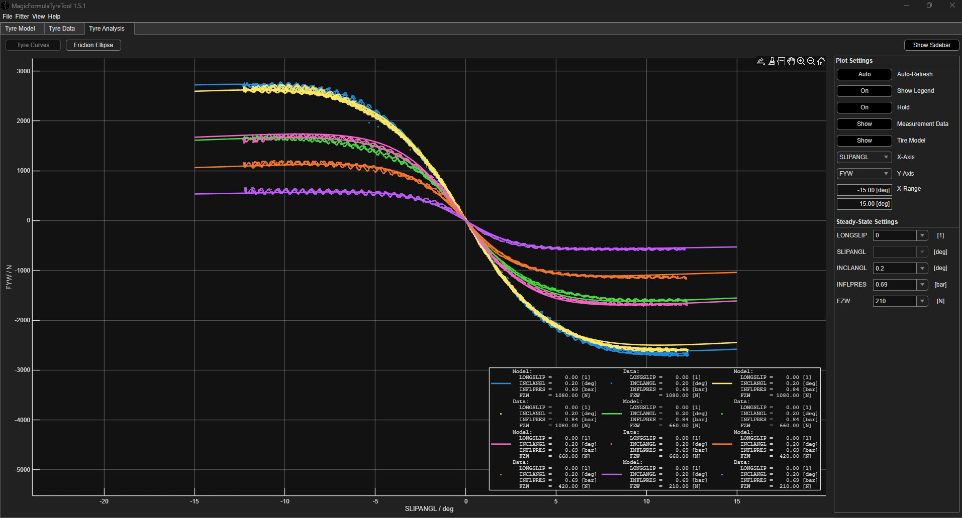
Fitted curves over measured dataLateral force against slip angle at four vertical loads. The solid lines are the fit; the speckle behind them is the measurement it was fitted to.
Querying the finished modelA small tool that loads a TIR file and returns Fy against slip angle at a chosen camber, pressure and load. Here that is 571 N/deg of cornering stiffness at 1000 N.
Finding a tyre with no dataPeak grip, stiffness and load sensitivity as three axes. The star is a compound with no test file; the dashed lines reach its three closest measured matches, at 31.1, 32.6 and 36.3 per cent distance.
The weighting behind the rankingSeven metrics with the reasoning written next to each. Peak grip takes 25 per cent, consistency and load sensitivity 20 each, and the two thermal terms 12.5 apiece.
Ranked resultThirteen candidates scored and sorted. The 16x7.5-10 R20 Hoosier comes out first on a total score of 4.9.
Cornering stiffness against vertical loadThree inflation pressures. At 50 kPa stiffness peaks near 750 N and falls away; at 97 kPa it is still climbing at 1500 N. This curve is what makes load sensitivity worth 20 per cent above.
Checking the bins before fittingData points per load-pressure-camber combination. Red bars fall under the threshold, so those bins are too thin to fit and are excluded rather than trusted.
Smoothing, chosen per channelMoving average, moving median or Savitzky-Golay with a settable window, because peak-preserving matters on some channels and outlier rejection on others.
Load cases to includeWhich vertical loads from the sweep go into a given fit: 210 to 1080 N here, with the zero-load run left out.
Raw channel browserAny two channels from a run file plotted against each other, which is how the data gets looked at before any of it is fitted.
Vertical load through a runThe load sweep as the rig applied it, read straight off the raw file.
Inflation pressure through a runChecked alongside load, because pressure drift through a run moves the fit if it is not binned out.
The simple tyre model it replacedA Pacejka call with a load-sensitive peak: D falls with vertical force through a1 and a2. Enough for early work, and the reason MF 6.1 was worth the effort.
Simple model against its targetLateral force against slip angle from the simple formula, laid over the curve it was matched to.
2 DOF

Quarter car: ride, damping and contact patch

MATLAB
Simulink
front and rear

One corner, two masses: sprung and unsprung, with the tyre as a spring down to the road. Road input is either a measured profile or a PSD-shaped random surface. Sweeping the damping coefficient traces RMS body acceleration against RMS damper velocity, so comfort and control are read off the same axis and the point where more damping stops buying ride quality is a number rather than an opinion.

The two-mass plantSpring and damper forces on the left, the two acceleration summations in the middle, and the tyre spring returning contact patch force at the bottom.
Where the body mode sitsFFT of sprung-mass acceleration. The peak is at 3.42 Hz, which is the number the spring rate was chosen to place.
Ride against controlRMS vertical acceleration falls, bottoms out near 1550 Ns/m and climbs again, while RMS damper velocity falls the whole way. The marked optimum is where the first curve turns.
Both ends of the sweepLow damping gives the bigger first peak and the quicker decay; high damping gives a lower peak that rings on far longer. Neither is free.
The damper curves themselvesForce against velocity, bump and rebound, front and rear, for a comfort tune and a contact-patch-force tune. Four settings compared on one axis.
The random road inputA PSD-shaped displacement input, used where a measured profile would make the result specific to one piece of tarmac.
Body acceleration responseSprung-mass acceleration through the run, the channel the RMS sweep integrates.
Output wiringThe seven channels the model publishes, including contact patch force, which is what the spring rate study is actually judged on.
Reference: contact patch force against spring ratePublished figure (Fig. 8.48) showing RMS contact patch force rising with spring rate across a road sweep. That is the trend the model's own sweep was checked against.
4 DOF

Pitch and heave

MATLAB
Simulink

Front and rear corners carried on one body, so heave and pitch are solved together rather than one at a time. The road is a physical track profile: discrete bumps at set distances rather than noise. That makes it easy to see how far the platform has settled before the next event arrives.

Four-state plantTwo unsprung corners under a sprung mass free in heave and pitch, with the geometry that converts the two corner deflections into body attitude.
The road as laid outBump heights of 50 to 150 mm at 10, 50, 100, 150 and 200 m, so each disturbance is isolated and the recovery between them is visible.
Pitch responseOne packet per bump. The 150 mm bump at 100 m takes the body to 0.23 rad and needs roughly a second to settle.
Heave responseThe same events read as vertical body movement, which is the half the driver feels through the seat rather than the steering.
4 DOF

Roll, and where the load transfer goes

MATLAB
Simulink
ARB in the loop

The roll pair of the same structure: a sprung mass in roll over two unsprung corners, with the anti-roll bar included rather than folded into an equivalent spring rate. The corner equation of motion splits load transfer three ways: what goes through the springs and bars, what goes through the roll centre and the links, and what the unsprung mass puts straight into the tyre. That is the split the calculator below was written to check.

Roll plantSprung mass in roll above, the two unsprung corners below, and the anti-roll bar force entering as its own term.
The corner equation of motionTyre force in, spring, damper and weight out, with the sprung and unsprung lateral terms entering through the roll centre height and the track. The elastic, geometric and unsprung split, written as blocks.
Roll angle to a step inputA step at three seconds, a brief overshoot the other way, then settled at 6.1 mrad and holding.
Unsprung corner displacementWhat the wheel does while the body rolls, which is where the tyre load change actually comes from.
2 DOF

Bicycle model

MATLAB
Simulink
15 parameters

Two states, yaw rate and sideslip, and the smallest model that will tell you whether the car understeers. Cornering stiffness is read against vertical load rather than fixed, so the balance still moves as the car loads up. This is the model the corner balance model grew out of, and the one its answers get sanity-checked against.

Two-state plantFront and rear slip angles, cornering stiffness lookups, and the yaw and lateral equations solved together.
Second revisionThe same model after the tyre call was swapped for a load-sensitive lookup rather than a constant.
Reference: steered angle against speedThe standard chart: understeer gradients from +1.0 to -1.0 deg/g about the neutral-steer line, with critical speed where the negative gradient runs to zero. The model's output is read against this.
Cornering stiffness against loadThe lookup the model uses, so the front and rear stiffnesses separate as weight shifts rather than staying where they started.
Yaw rate response, parameter sweptTwenty runs from 105 to 200. The steady-state yaw rate is unchanged at 22 deg/s; what moves is how quickly the car gets there.
3 DOF

Braking

MATLAB
Simulink
12 parameters

Longitudinal braking with wheel rotation at each axle. Pedal force runs through master cylinder area, brake bias, clamp force and rotor radius to a torque at each wheel, so bias is a setting you change and immediately see in the load split. The run here reaches 140 km/h, coasts, and brakes hard at three seconds.

Braking plantLongitudinal equation, wheel rotation at both axles, and the load transfer term that feeds the tyre forces.
Pedal to wheel torquePedal position, maximum pedal force, bias split, master cylinder area, clamp force, then rotor radius. Each one is a real number rather than a single gain.
Equations of motionThe longitudinal and rotational states laid out as built.
The I-curveIdeal front against rear brake force at three speeds, with the fixed 0.725 bias line through it. Where the straight line sits above the curve, the front locks first.
Velocity140 km/h down to a stop. Braking starts at three seconds from 104.7 km/h and the car is stationary at 5.88 s.
Stopping distance101.6 m covered before the brakes come on, 138.3 m by the time it stops, so 36.7 m of braking.
DecelerationA peak of -17.4 m/s² the instant the pedal goes down, easing to about -8.5 as speed and downforce fall away.
Front normal load2750 N at the moment of application, against roughly 1990 N coasting. That is the load the front tyre model is being asked about.
Rear normal loadThe other side of the same transfer: 1890 N down to 1108 N, which is how little there is left to brake with at the back.
2 DOF

Acceleration

MATLAB
Simulink
motor map

The straight-line run. A two-dimensional motor map is looked up on RPM and throttle, scaled by maximum motor torque and geared to the wheel, then held against rear slip ratio and longitudinal load transfer. It publishes the three channels that matter for gearing: acceleration, velocity and distance. Slip ratio, motor RPM and vertical force come out alongside them.

Model interfaceInitial velocity and throttle position in; acceleration, velocity, distance, rear slip ratio, motor RPM, gear and vertical force out.
Motor map lookupGear ratio and wheel speed to RPM, RPM and throttle into the two-dimensional map, normalised torque scaled by the motor's peak.
Full plantThe traction and load transfer side of the model, downstream of the motor map.
Longitudinal accelerationWhat the tyre will actually take, rather than what the motor would give.
VelocityThe speed trace the gear ratio is chosen against.
Distance coveredDistance against time, so the event can be read straight off the trace.
3 mechanisms

Lateral load transfer calculator

Excel
SI throughout
Milliken §18.4

The Milliken neutral-roll-axis method, re-expressed in SI and laid out so every input is visible. Mass, CG height, track, roll stiffness and roll centre heights go in; out comes the load transfer split by mechanism, the roll gradient, the front-to-rear distribution, and an inside-wheel lift check. It seeds the Simulink models, and gives a hand calculation to check them against. The moment balance line at the bottom is there to catch the small-angle assumption drifting.

Total mass290 kg
Wheelbase1.530 m
CG height0.300 m
Track, front / rear1.220 / 1.180 m
Roll stiffness, front / rear12,000 / 18,000 N·m/rad
Load transfer distribution44.5 % front
Roll gradient1.28 deg/g
Inputs290 kg at 15 m/s², a 1.530 m wheelbase and a 0.300 m CG, with 12,000 N·m/rad of front roll stiffness against 18,000 at the rear.
Outputs44.5 per cent of lateral load transfer at the front, a 1.28 deg/g roll gradient, 1.96 deg of body roll, and the moment balance closing to 99.94 per cent.
Split by mechanism, as a shareThe front puts 26.4 per cent of its transfer through geometry; the rear only 4.8. That difference is the roll centre heights, and it is a balance adjustment that costs nothing in spring rate.
Split by mechanism, in newtonsThe same result in force: 485 N at the front against 604 N at the rear, 1089 N in total.
The method it implementsMilliken and Milliken, Race Car Vehicle Dynamics, section 18.4. Every equation in the sheet is taken from that derivation.

The map it was all planned from

Nineteen models down the top, twenty-seven measurements down the side, and a cross in every cell where one needs the other. It was written before the models were, so the test plan knew what to go and measure and nothing ended up built on a guess.

Vehicle dynamics model mapAll nineteen models against the parameters each one needs. The full 14 DOF car wants 35 of them; the 9 DOF corner balance model wants 26. Tyre vertical stiffness is the most-wanted measurement on the sheet, needed by fourteen models.

Where the theory came from

A vehicle dynamics course worked through alongside the build. The derivations behind the Simulink blocks above start here: slip angles, the braking balance, the pitch equations.

Lateral dynamics: the bicycle modelFront and rear slip angles under the small-angle approximation, and the vehicle slip angle at the CG. These are the three expressions the bicycle model is built out of.
BrakingThe longitudinal module behind the braking model.
Pitch, three degrees of freedomThe pitch derivation that the pitch and heave model extends to four.

Get in touch

Happy to walk through any of these.